Gramener Case Study
Gramener is the largest online loan marketplace, facilitating personal loans, business loans, and financing of medical procedures. Borrowers can easily access lower interest rate loans through a fast online interface. Like most other lending companies, lending loans to ‘risky’ applicants is the largest source of financial loss (called credit loss).
The credit loss is the amount of money lost by the lender when the borrower refuses to pay or runs away with the money owed. In other words, borrowers who default cause the largest amount of loss to the lenders. In this case, the customers labelled as 'charged-off' are the 'defaulters'. If one is able to identify these risky loan applicants, then such loans can be reduced thereby cutting down the amount of credit loss. Identification of such applicants using EDA is the aim of this case study.
In other words, the company wants to understand the driving factors (or driver variables) behind loan default, i.e. the variables which are strong indicators of default. The company can utilise this knowledge for its portfolio and risk assessment.
In this case study, we will apply EDA (Exploratory Data Analysis) Techniques to develop understanding of risk analytics and finacial service. With this EDA, we will try to understand how to minimise risk of loosing money while lending money to customer.
Business Requirement
Gramener consumer finance company which specialises in lending various types of loans to urban customers. When the company receives a loan application, the company has to make a decision for loan approval based on the applicant’s profile. Two types of risks are associated with the bank’s decision:
If the applicant is likely to repay the loan, then not approving the loan results in a loss of business to the company
If the applicant is not likely to repay the loan, i.e. he/she is likely to default, then approving the loan may lead to a financial loss for the company
The data given in the dataset contains the information about past loan applicants and whether they ‘defaulted’ or not. The aim is to identify patterns which indicate if a person is likely to default, which may be used for taking actions such as denying the loan, reducing the amount of loan, lending (to risky applicants) at a higher interest rate, etc.
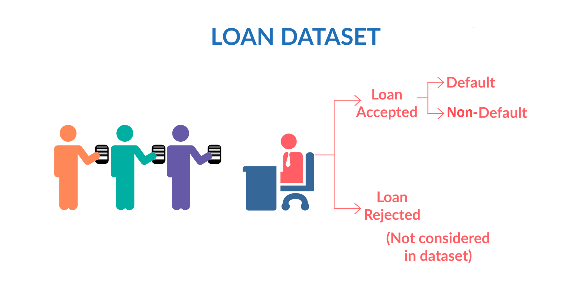
When a person applies for a loan, there are two types of decisions that could be taken by the company:
Loan accepted: If the company approves the loan, there are 3 possible scenarios described below:
Fully paid: Applicant has fully paid the loan (the principal and the interest rate)
Current: Applicant is in the process of paying the instalments, i.e. the tenure of the loan is not yet completed. These candidates are not labelled as 'defaulted'.
Charged-off: Applicant has not paid the instalments in due time for a long period of time, i.e. he/she has defaulted on the loan
Loan rejected: The company had rejected the loan (because the candidate does not meet their requirements etc.). Since the loan was rejected, there is no transactional history of those applicants with the company and so this data is not available with the company (and thus in this dataset)
## Import Python Modeules
import pandas as pd
import numpy as np
import matplotlib.pyplot as plt
import seaborn as sns
Data loading and Cleaning
Next we will load the loan csv and then do the following
1) find out which all columns are having null/NaN values, find all these columns and drop them as they dont give any inputs.
2) use the null value dataframe to find which columns are null and filter out them from main data.
loan_data = pd.read_csv('./loan.csv',low_memory=False)
print('size of data with id as unique column {}'.format(loan_data.id.count()))

# print(loan_data.isnull().sum()/len(loan_data.index))
nullSeries = loan_data.isnull().sum()/len(loan_data.index)
null_data = pd.DataFrame(nullSeries,columns=['nullindex'])
nonNullCol = list(null_data.loc[null_data.nullindex!=1.0].index)
loan_data = loan_data[nonNullCol]

print(loan_data.shape)
loan_data.head()
d = pd.DataFrame(loan_data.isnull().sum()/len(loan_data.index),columns=['nullper'])
d = d.loc[d.nullper > 0]

e = pd.DataFrame(loan_data[loan_data.loan_status == 'Charged Off'].isnull().sum()/len(loan_data[loan_data.loan_status == 'Charged Off'].index),columns=['co_nullper'])
e = e.loc[e.co_nullper > 0]

pd.concat([d,e],axis=1)
Now we will start data cleaning column wise and since the below columns have large % of null values.
1) 'mths_since_last_record' --> 92% null values,
2) 'next_pymnt_d' --> 97% null values
variables with less business significance 3) member_id --> because its a random number and we already have id as unique key. No inputs for making Charged off decisions
4) funded_amnt_inv --> The loan is funded, and investers are not going to get money back :)
5) sub_grade --> redundant information with grade column
6) issue_d --> the loan is already funded
7) zip_code --> Unable to process the data to a meaning form as it requires lot of patience.
8) out_prncp --> It kind of gives information to current loan rather than charged off cases.
9) out_prncp_inv --> It kind of gives information to current loan rather than charged off cases.
10) total_pymnt_inv --> redundant columns WRT to total_pymnt
11) total_rec_prncp, total_rec_int --> It kind of gives information to current loan rather than charged off cases.
replace the text columns with some knows strings instead of dropping the rows for it. then for the remaining columns which have null values we can drop the corresponding rows.
loan_data = loan_data.drop(['mths_since_last_record','next_pymnt_d','member_id','funded_amnt_inv','sub_grade'\
                           ,'issue_d','zip_code','out_prncp','out_prncp_inv','total_pymnt_inv','total_rec_prncp'\
                            , 'total_rec_int' ], axis=1)
Analysis to check for mths_since_last_delinq releaved that for the column the nulls values are for cases charged off, hence replacing that column with std or median should be fine. Prefering std value so that we dont put too much penalty on the 4% null values which are in non-default cases.
a = loan_data[loan_data.loan_status == 'Charged Off'].mths_since_last_delinq.dropna()
print(a.describe([0.1,0.25,0.75,0.9,0.95,0.97,0.99]))

## identify lower and upper bound and remove outliers
IQR = a.quantile(0.75) - a.quantile(0.25)
step = 1.0 * IQR
lowerbound = 0 if (a.quantile(0.25) - step) < 0 else (a.quantile(0.25) - step)
upperbound = a.quantile(0.75) + step
print(lowerbound)
print(upperbound)

a = a[a < upperbound]
plt.figure(figsize=(17,5))
plt.subplot(131)
sns.distplot(a)
plt.subplot(132)
sns.boxplot(y = a)
plt.subplot(133)
plt.hist(a)
#plt.yscale('log')
plt.show()

a.describe([0.1,0.25,0.75,0.9,0.95,0.97,0.99])

Now we will start conditioning/value treatments for the respective columns after looking sample data from each column, like remove the % from float percent values, impute values And specifically for empoyee experience convert the categories into 10 buckets
loan_data.mths_since_last_delinq.fillna(22.5,inplace=True)
loan_data.emp_title.fillna('unknown_emp_title', inplace=True)
loan_data.desc.fillna('unknow_desc',inplace=True)
loan_data.title.fillna('unknow_title',inplace=True)
type(loan_data['emp_length'][0])
loan_data["emp_length"] = loan_data["emp_length"].astype(str)
# treating   emp_length as categorical by converting to nominal variable
loan_data["emp_length"] = loan_data["emp_length"].apply(lambda x: '0' if (x == 'n/a' or x == '< 1 year') else x)
loan_data["emp_length"] = loan_data["emp_length"].apply(lambda x: x.replace("years", "").replace("year", "").replace("+","").replace(">","").strip())


print('rows having number of null values {}'.format(set(loan_data.isnull().sum(axis=1))))
print('columns having number of null values {}'.format(set(loan_data.isnull().sum())))
loan_data = loan_data.dropna()

print(loan_data.shape)
d = pd.DataFrame(loan_data.isnull().sum()/len(loan_data.index),columns=['nullper'])
d = d.loc[d.nullper > 0]

e = pd.DataFrame(loan_data[loan_data.loan_status == 'Charged Off'].isnull().sum()/len(loan_data[loan_data.loan_status == 'Charged Off'].index),columns=['co_nullper'])
e = e.loc[e.co_nullper > 0]

pd.concat([d,e],axis=1)
#uncomment this code to see sample value for each column.
# cols = loan_data.columns.values
# for colName in cols:
#     print(loan_data[colName].head(2))

loan_data['term'] = loan_data.term.apply(lambda x: int(x[0:3]))
loan_data['int_rate'] = loan_data.int_rate.apply(lambda x: float(x.strip('%')))
loan_data['revol_util'] = loan_data.revol_util.apply(lambda x: float(x.strip('%')))

print(loan_data.shape)
loan_data.head()
invSet = ["","n/a","N/A"]
cols = loan_data.columns.values
dataDict = {'int64':[],'float64':[],'object':[]}
for colName in cols:
#     print('column contain invalid values {0}:{1}'.format(colName,loan_data.loc[loan_data[colName].isin(invSet)].empty))
    dataDict[str(loan_data[colName].dtype)].append(colName)

print('probable Categorical values')
print(dataDict['object'],'\n')
print('probable Continuous values')
print(dataDict['int64'],'\n')
print(dataDict['float64'],'\n')
# loan_data.head()
1) Again use the categorical value first and then check if each category is a single constant value and then we can plan to exclude that as that will not give us any information
2) Build a dataframe on the univariate analysis for all the comtinuous variables, and then check if the columns is having single value like 0.0 or 0 and drop them as they dont give us information for analysis
3) Filter out the desc, url , title and emp_title as they can be considered for sentiment analysis kind of overwork here.
# seeing from popular categories for which we can check on the analysis.
catColList = list()
for eachCat in dataDict['object']:
    if(eachCat not in ['desc','url','title','emp_title']):
#         print('{0} : {1}'.format(eachCat,set(loan_data[eachCat].unique())))
        if(len(loan_data[eachCat].unique()) > 1):
            catColList.append(eachCat)

#TODO for each continous column create the table of description and append the values to check how the data is changing per col
quantRange = [0.1,0.25,0.75,0.9,0.95,0.97,0.99]
condf = pd.DataFrame()
for eachCol in dataDict['int64']:
    if(eachCol not in ['id','member_id']):
        a = pd.DataFrame(loan_data[[eachCol]].describe(quantRange))[1:]#excluding the count as we are aware of that metric
        condf = pd.concat([a,condf], axis=1)

for eachCol in dataDict['float64']:
    a = pd.DataFrame(loan_data[[eachCol]].describe(quantRange))[1:]#excluding the count as we are aware of that metric
    condf = pd.concat([a,condf], axis=1)

#for univariate analysis on which has constant value might not have any inputs to be given for EDA (but can be considered for modelling)
# print(condf.head(12))
condf.to_csv('./univariate_column_meta_data.csv')
nunique = condf.apply(pd.Series.nunique)
cols_to_drop = nunique[nunique == 1].index
print('columns having unique/single value {}'.format(cols_to_drop))
condf = condf.drop(cols_to_drop, axis=1)

reqColList = list(['id']) + list(catColList) + list(condf.columns.values)
loan_data = loan_data[reqColList]
loan_data.to_csv('./loan_cleanedup.csv')
print(loan_data.columns.values)
loan_data.head()
loan_data.columns
loan_data['loan_status'].value_counts()
We can see that, most of the loans comprises of fully_paid status, while there is some chunk which is current running loans. We can not analyse based on current loans as they have not yet defaulted so lets get rid of them.
loan_data = loan_data[loan_data['loan_status'] != 'Current']
Univariate Analysis
1) Perform the univariate (for categorical and continous) indivdual columns, like removal of outliers, finding the tuning the mean and 50th quantile difference
2) Derrive new columns as well as and when required.
#create some common functions for performing univariate analysis
#For funded_amount
def outlierranges(loan_data,col_name,exp):
    ## identify lower and upper bound and remove outliers
    IQR = loan_data[col_name].quantile(0.75) - loan_data[col_name].quantile(0.25)
    step = exp * IQR
    lowerbound = 0 if (loan_data[col_name].quantile(0.25) - step) < 0 else (loan_data[col_name].quantile(0.25) - step)
    upperbound = loan_data[col_name].quantile(0.75) + step
    print('lower bound ', lowerbound)
    print('upper bound ', upperbound)
    return lowerbound,upperbound

def plotContinousVar(loan_data,col_name,logScale):
    plt.figure(figsize=(20,5))
    plt.subplot(131)
    sns.distplot(loan_data[col_name])
    plt.subplot(132)
    sns.boxplot(y = loan_data[col_name])
    plt.subplot(133)
    plt.hist(loan_data[col_name])
    if(logScale == True):
        plt.yscale('log')
    plt.show()

def getDefaultPercentageDF(loan_data, column_name):
    #calculate total count per category
    count_df = loan_data[['id',each]].groupby(each, as_index=False)\
                                             .count()\
                                             .sort_values(by='id',ascending=False)
    count_df = count_df.rename(index=str,columns={'id':'total_count'})

    #calculate charged off count per category
    co_count_df = loan_data[['id','loan_status',each]].loc[loan_data.loan_status ==1]\
                                                              .groupby([each,'loan_status'],as_index=False)\
                                                              .count()
    co_count_df = co_count_df.rename(index=str,columns={'id':'co_count'})

    #merge the two categories and calculate the derived column for charged off % and see which is having high variance
    final_df = pd.merge(count_df,co_count_df,on=each)
    final_df['default %'] = round((final_df.co_count/final_df.total_count)*100,2)
    return count_df,final_df
## Lets convert loan_status to numeric field for summarization
loan_data['loan_status'] = loan_data['loan_status'].apply(lambda x: 0 if x=='Fully Paid' else 1)

# converting loan_status to integer type
loan_data['loan_status'] = loan_data['loan_status'].apply(lambda x: pd.to_numeric(x))

# summarising the values
loan_data['loan_status'].value_counts()
Start Anayzing the categorical variables, but first doing a coutn plot of loans applied for each category compared to the charged off % of each category.
While analysing the categorical column, we see some categories in count plot and some categories in missing default %plot as the reason would be that they are not applicable for "charged off" cases
cat_col_list = ['emp_length', 'home_ownership', 'verification_status', 'purpose','addr_state', 'grade',\
                'pub_rec_bankruptcies','term','pub_rec','policy_code','delinq_2yrs','open_acc','total_acc']

for each in cat_col_list:
    count_df, final_df = getDefaultPercentageDF(loan_data,each)

    #plot to understand where the maximum loans are lended/funded
    plt.figure(figsize=(20,5))
    plt.subplot(121)
    sns.pointplot(x=each, y="total_count", data=count_df)
    plt.xticks(rotation=90)

    plt.subplot(122)
    sns.pointplot(x=each, y="default %", data=final_df)
    plt.xticks(rotation=90)

    plt.show()
    print('--------------------------------------------------------------------------------------------------------------------')


# Lets plot default rates across various categorical features of the loan to understand the impact

for each in cat_col_list:
    plt.figure(figsize=(16, 6))
    sns.barplot(x=each, y='loan_status', data=loan_data)
    plt.show()


From the above plots we can clearly see the following:
- Emp length -> No much variation in default rates
- Home ownership -> no visible trend
- verification status -> Verified loans are more dafaulted then other categories
- purpose -> Small business defaults more than other cat
- states -> not looking much useful so far
- grades -> there is incresing number of defaults across categories from A to G
- pub_rec_bankrupcies -> increasing treand with no of bank rupcies
- term -> more defaults on longer term loans
- nuber_of_der_pub_records -> more defaults with 1
- policy_code -> not useful
- delinq_2years -> increasing trends
- open_acc -> most defaults with more number of open accounts
- total_acc -> more defaults with large number of total accounts
#int_rate
plotContinousVar(loan_data,'int_rate',False)
print(condf['int_rate'])

#since the int_rate dist plot has some bins to it, we can create probably categories out of it.
def int_rate_grp(int_rate):
    if(int_rate <= 8.0):
        return "low"
    elif (int_rate > 8.0 and int_rate <= 18.0):
        return "medium"
    else:
        return "high"

loan_data['int_rate_grp'] = loan_data['int_rate'].apply(int_rate_grp)

## feature: installment
## Description: The monthly payment owed by the borrower if the loan originates.

plotContinousVar(loan_data,'installment',False)
print(condf['installment'])
lower,upper = outlierranges(loan_data,'installment',1.5)

# loan_data = loan_data.loc[loan_data['installment'] < upper]
# loan_data.installment.describe()
loan_data.hist(column='installment',
                  figsize=(20,10),
                  bins=50,
                  color="blue",
                  range= (0,900))
plt.show()


## feature: annual_inc
## Description: The self-reported annual income provided by the borrower during registration.

plotContinousVar(loan_data,'annual_inc',True)
plt.figure(figsize=(20,5))

print(condf['annual_inc'])
lower,upper = outlierranges(loan_data,'annual_inc',1.5)

## Lets check number of records with annual income > 140000
#loan_data = loan_data.loc[loan_data['installment'] < upperbound]
#loan_data.shape
print((loan_data.loc[loan_data['annual_inc'] > upper].shape[0] / loan_data.shape[0]) * 100)

#We have 1.89% outliers with annual income. Lets remove these outliers-
loan_data.hist(column='annual_inc',
                  figsize=(20,10),
                  bins=50,
                  color="blue",
                  range= (0,200000))
plt.show()
loan_data = loan_data.loc[loan_data['annual_inc'] < upper]
loan_data.annual_inc.describe()


## feature: dti
## Description: A ratio calculated using the borrower’s total monthly debt payments on the total debt obligations,
## excluding mortgage and the requested LC loan, divided by the borrower’s self-reported monthly income.

plotContinousVar(loan_data.loc[loan_data.loan_status==1],'dti',False)
print(condf['dti'])

## feature: revol_util
## Description: Revolving line utilization rate,
## or the amount of credit the borrower is using relative to all available revolving credit.

plotContinousVar(loan_data,'revol_util',False)
print(condf['revol_util'])

## feature: total_pymnt
## Description: Payments received to date for total amount funded.

plotContinousVar(loan_data,'total_pymnt',False)
print(condf['total_pymnt'])
lower,upper = outlierranges(loan_data,'total_pymnt',1.5)

## lets see the percentage of outlier records
print((loan_data[loan_data['total_pymnt'] > upper].shape[0] / loan_data.shape[0]) * 100)
loan_data = loan_data[loan_data['total_pymnt'] < upper]
loan_data.total_pymnt.describe()

loan_data.loc[loan_data.loan_status==1].hist(column='total_pymnt',
                  figsize=(20,10),
                  bins=50,
                  color="blue",
                  range= (0,30000))
plt.show()


# total_rec_late_fee	Late fees received to date

plotContinousVar(loan_data,'total_rec_late_fee',True)
print(condf['total_rec_late_fee'])
lower,upper = outlierranges(loan_data,'total_rec_late_fee',1.5)

## lets see the percentage of outlier records
print((loan_data[loan_data['total_rec_late_fee'] > upper].shape[0] / loan_data.shape[0]) * 100)
# loan_data1 = loan_data[loan_data['total_rec_prncp'] < upper]
# print(loan_data1.total_pymnt.describe())
# print(loan_data1.shape)

# Univariate Analysis for total_rec_late_fee field
# Mean is higher than Median value because of Outliers present in the data.
# 90 to 100 percentile contains around 100% of the Value.
# So, Median is the representative value for this column.

# Density Plot for this column shows a Spike at 0 because 0 to 90 percentile contains just 0.
# No Outliers
# Histogram Shows the frequency of different values.
loan_data.loc[loan_data.loan_status==1].hist(column='total_rec_late_fee',
                  figsize=(20,10),
                  bins=50,
                  color="blue",
                  range= (0,150))
plt.show()


# recoveries	post charge off gross recovery

plotContinousVar(loan_data,'recoveries',True)
print(condf['recoveries'])

loan_data.loc[loan_data.loan_status==1].hist(column='recoveries',
                  figsize=(20,10),
                  bins=50,
                  color="blue",
                  range= (0,20000))
plt.show()


# collection_recovery_fee	post charge off collection fee

plotContinousVar(loan_data.loc[loan_data.loan_status==1],'collection_recovery_fee',True)
print(condf['collection_recovery_fee'])

loan_data.loc[loan_data.loan_status==1].hist(column='collection_recovery_fee',
                  figsize=(20,10),
                  bins=50,
                  color="blue",
                  range= (0,6000))
plt.show()


# last_pymnt_amnt	Last total payment amount received

plotContinousVar(loan_data,'last_pymnt_amnt',True)
print(condf['last_pymnt_amnt'])

loan_data.loc[loan_data.loan_status==1].hist(column='last_pymnt_amnt',
                  figsize=(20,10),
                  bins=50,
                  color="blue",
                  range= (0,30000))
plt.show()


# loan_amnt	The listed amount of the loan applied for by the borrower.
#If at some point in time, the credit department reduces the loan amount, then it will be reflected in this value.

plotContinousVar(loan_data,'loan_amnt',False)
print(condf['loan_amnt'])
lower,upper = outlierranges(loan_data,'loan_amnt',1.5)

## lets see the percentage of outlier records
print((loan_data[loan_data['loan_amnt'] > upper].shape[0] / loan_data.shape[0]) * 100)
loan_data = loan_data[loan_data['loan_amnt'] < upper]
print(loan_data.total_pymnt.describe())
print(loan_data.shape)

From the loan amount distribution we can see that median (50th percentile) of the loan amount is 10000. Lets use this make some bins and analyse the default rates across different amounts
def loan_amount(n):
    if n < 5000:
        return 'low'
    elif n >=5000 and n < 15000:
        return 'medium'
    elif n >= 15000 and n < 25000:
        return 'high'
    else:
        return 'very high'

loan_data['loan_amnt_bin'] = loan_data['loan_amnt'].apply(lambda x: loan_amount(x))
## Lets plot and see default rates across these categories of loan amounts
plt.figure(figsize=(16, 6))
sns.barplot(x='loan_amnt_bin', y='loan_status', data=loan_data)
plt.show()

We can clearly see that higher the loan amount, more are the chances of default.
# revol_bal	Total credit revolving balance

plotContinousVar(loan_data,'revol_bal',True)
print(condf['revol_bal'])
lower,upper = outlierranges(loan_data,'revol_bal',1.5)

## lets see the percentage of outlier records
print((loan_data[loan_data['revol_bal'] > upper].shape[0] / loan_data.shape[0]) * 100)

loan_data.loc[loan_data.loan_status==1].hist(column='revol_bal',
                  figsize=(20,10),
                  bins=50,
                  color="blue",
                  range= (0,160000))
plt.show()


#Derive the ratio of savings that a borrower can have by doing for math (annual_inc/12)-installment and see how the variable

loan_data['month_saved_amnt'] = round((loan_data['annual_inc']/12)-loan_data['installment'],2)
print(loan_data.month_saved_amnt.describe([0.25,0.75,0.9,0.95,0.99]))

plotContinousVar(loan_data.loc[loan_data.loan_status==1],'month_saved_amnt',True)
lower,upper = outlierranges(loan_data.loc[loan_data.loan_status==1],'month_saved_amnt',1.5)

## lets see the percentage of outlier records
print((loan_data[loan_data['month_saved_amnt'] > upper].shape[0] / loan_data.shape[0]) * 100)

loan_data.loc[loan_data.loan_status==1].hist(column='month_saved_amnt',
                  figsize=(20,10),
                  bins=50,
                  color="blue",
                  range= (0,12000))
plt.show()


Date type analysis to check on the charged off % and total amount funded
getFirst = lambda x: str(x.split('-')[0])
getSecond = lambda x: str(x.split('-')[1])

loan_data['earliest_cr_line_month'] = loan_data['earliest_cr_line'].apply(getFirst)
loan_data['earliest_cr_line_year'] = loan_data['earliest_cr_line'].apply(getSecond)
loan_data['last_pymnt_month'] = loan_data['last_pymnt_d'].apply(getFirst)
loan_data['last_pymnt_year'] = loan_data['last_pymnt_d'].apply(getSecond)
loan_data['last_credit_pull_month'] = loan_data['last_credit_pull_d'].apply(getFirst)
loan_data['last_credit_pull_year'] = loan_data['last_credit_pull_d'].apply(getSecond)

date_cols = ['earliest_cr_line_month','earliest_cr_line_year','last_pymnt_month',\
             'last_pymnt_year','last_credit_pull_month','last_credit_pull_year']

for each in date_cols:
    count_df, final_df = getDefaultPercentageDF(loan_data,each)

    #plot to understand where the maximum loans are lended/funded
    plt.figure(figsize=(20,5))
    plt.subplot(121)
    sns.pointplot(x=each, y="total_count", data=count_df)
    plt.xticks(rotation=90)

    plt.subplot(122)
    sns.pointplot(x=each, y="default %", data=final_df)
    plt.xticks(rotation=90)

    plt.show()
    print('--------------------------------------------------------------------------------------------------------------------')

print(loan_data.shape)


Inferences from univariate analysis
Selecting the variables which might give good insigths on the data
1) emp_length --> we can see that higher exp people are showing more defaults
2) home_ownership --> 1 category is showing 19% of default, use in bivariate
3) verification_status --> 1 category i.e. Verified is shwoing 16% of defaults
4) purpose --> Small business categories is showing > 25% of defaults
5) state --> observed good power law distribution for states CA, NY, FL, TX
6) grade --> some grades are showing around 30% of default
7) last_pymnt_year --> some years show around 20% - 40% defaults, which includes year 2009 which was recession
8) int_rate --> split into multiple bins and analyzed further
9) month_saved_amnt --> business combined data WRT to installment and annual_inc which were showing good normal distributions
10) total_payment , revol_bal, loan_amnt --> Showing promising distribution for analysis
dropping the below variables which were kind of showing less significance on Charged Off data.
1) revol_util,dti --> kind of flat distribution/histogram plots
2) total_rec_late_fee,recoveries,collection_recovery_fee,last_pymnt_amnt --> all of them show 0 values for the chanrged off loan_data
3) earliest_cr_line --> power law distribution shows that LSH and RHS are only showing max loans provided, and center part low number of loans and less data
4) last_pymnt_d -- > converted to last last_pymt_year
5) last_credit_pull_d --> giving same insights as that of last_payment_year
Segmented Univariate Analysis
From the univariate analysis we saw that there are some clear preditors for loan defaults like loan purpose, duration, interest rate, annual income, grade, loan amount.
from the business point of view, its always makes sense to have analysis on the purpose of the loan. Lets see is we can get some more insights from the purpose itself.
# We have already seen that small business have more default rates than other categories in univariate analysis.
# Lets see which other purposes makes more sense and then examin them.
plt.figure(figsize=(16, 10))
sns.barplot(x='loan_status',y='purpose', data=loan_data, palette="Blues_d")
plt.show()

## Also check the most used type of loans
plt.figure(figsize=(16, 10))
sns.countplot(y="purpose", data=loan_data, palette="Blues_d")

loan_data['purpose'].value_counts()
Now making use of the above two plots, we can see that most of the defaults are happening across
- small business
- renewable energy
- educational
- moving
- medical ### Most of the loans are from the categories:
- debt_consolidation
- credit_card
- others
- home_improvements
- major_purcases
Lets now check the distribution of default percentage across identified features from univariate analysis i.e.
emp_length, home_ownership,verification_status, grade, last_pymnt_year, int_rate_grp, emp_length, loan_amnt_bin,
seg_features = ["emp_length", "home_ownership","verification_status", "grade", "last_pymnt_year", "int_rate_grp", "emp_length", "loan_amnt_bin"]

# plots for segmented analysis
for feature in seg_features:
    plt.figure(figsize=[16, 10])
    sns.barplot(x=feature, y="loan_status", hue='purpose', data=loan_data)
    plt.show()


Bivariate Analysis
# Compute the correlation matrix
corr = loan_data[['month_saved_amnt','total_pymnt','loan_amnt','revol_bal','revol_util','dti',\
                  'total_rec_late_fee','recoveries','last_pymnt_amnt']].corr()

# Generate a mask for the upper triangle
mask = np.zeros_like(corr, dtype=np.bool)
mask[np.triu_indices_from(mask)] = True

# Set up the matplotlib figure
f, ax = plt.subplots(figsize=(11, 9))

# Generate a custom diverging colormap
cmap = sns.diverging_palette(220, 10, as_cmap=True)

# Draw the heatmap with the mask and correct aspect ratio
sns.heatmap(corr, mask=mask, cmap=cmap, vmax=.3, center=0,
            square=True, linewidths=.5, cbar_kws={"shrink": .5})
plt.show()

#comparing the home ownership and purpose (Bivariate analysis on categorical values)
# import itertools
charof_df = loan_data
ana_cat_cols = ['emp_length','home_ownership','verification_status','purpose','addr_state','grade','last_pymnt_year','int_rate_grp']
ana_can_cols = ['month_saved_amnt','total_pymnt','loan_amnt','revol_bal']

# for subset in itertools.combinations(cat_col_list_1, 2):
for cat_col in ana_cat_cols:
    for conti_col in ana_can_cols:

        ptab = pd.pivot_table(charof_df,index=[cat_col], values=[conti_col],columns=['loan_status'],aggfunc=np.median)
        ptab.plot(kind='bar',figsize=(10,5),stacked=True)
        plt.xticks(rotation=45)
        plt.title('Median Value Plot of x:{0} vs y:{1}'.format(cat_col,conti_col))
#         plt.yscale('log')
        plt.grid()

        ptab1 = pd.pivot_table(charof_df,index=[cat_col], values=[conti_col],columns=['loan_status'],aggfunc=np.sum)
        ptab1.plot(kind='bar',figsize=(10,5),stacked=True)
        plt.xticks(rotation=45)
        plt.title('Total sum Plot of x:{0} vs y:{1}'.format(cat_col,conti_col))
        plt.yscale('log')
        plt.grid()

        plt.show()


#Perform the co-relation and head map analysis of the continuous variable

ptab2 = pd.pivot_table(charof_df,index=['purpose','int_rate_grp'], values=['loan_amnt'],columns=['loan_status'],aggfunc=np.sum)
ptab2.plot(kind='bar',figsize=(10,5),stacked=True)
plt.xticks(rotation=90)
plt.title('Total sum Plot of x:{0} vs y:{1}'.format(cat_col,conti_col))
plt.yscale('log')
plt.grid()
plt.show()
